5. Magnetic field models and units

We have support for different field models for planets. They are listed below:

• Mercury :

  • Anderson et al. 2012

  • Thébault et al. 2018

  • Wardinski et al. 2019

• Earth : IGRF 13, Alken et al. 2021

• Jupiter :

  • VIP4, Connerney et al. 1998

  • JRM09, Connerney et al. 2018

  • JRM33, Connerney et al.

• Saturn :

  • Cassini SOI, Burton et al. 2009

  • Cassini 11, Dougherty et al. 2018

  • Cassini 11+, Cao et al. 2020

• Uranus : Connerny et al. 1987

• Neptune : Connerny et al. 1991

• Ganymede: Kivelson et al. 2002

A list of models and keywords for them can be obtained using the get_models function. For example:

In [1]: from planetmagfields import get_models

In [2]: get_models("jupiter")
Out[2]: array(['jrm09', 'jrm33', 'vip4'], dtype='<U5')

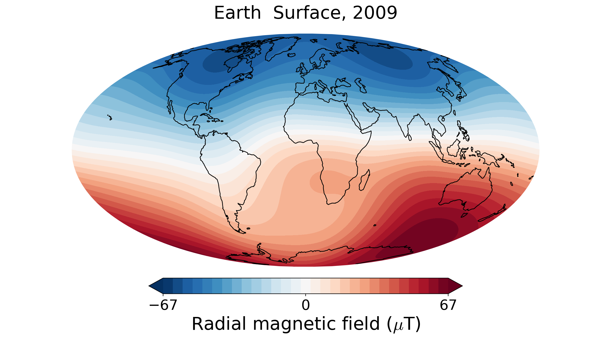
In case of Earth, a special argument year is also used to provide a year between 1900 to present day. This uses the IGRF13 model to compute a linear secular variation and extrapolate to the desired year. For example, the code below

In [1]: from planetmagfields import Planet

In [2]: p = Planet(name='earth',year=2009)
Planet: Earth
Model: igrf13
l_max = 13
Dipole tilt (degrees) = -10.500800
Year = 2009

In [3]: p.plot(r=1)

produces the surface magnetic field in the year 2009.

5.1. Units

In physical space, i.e., while plotting or extrapolating and obtaining the three components of the field \(B_r,B_\theta,B_\phi\), the default units are microTeslas. This can be changed while calling the planetmagfields.Planet class:

In [1]: from planetmagfields import Planet

In [2]: p = Planet(name='earth',year=2009,units='Gauss') #Will produce Br plots in Gauss

For spectral space, such as Gauss coefficients \(g_l^m\) and \(h_l^m\) (see section Mathematics) and Lowes spectrum (section Planet.spec()) are always in nanoTeslas (nT).