2. Features and examples

2.1. The Planet class

This gives access to all the relevant properties of a planet and has methods to plot the field and write a vts file for 3D visualization. Usage:

from planetmagfields import Planet
p = Planet(name='earth')

This displays the some information about the planet

Planet: Earth
l_max = 13
Dipole tilt (degrees) = -9.410531

and gives access to variables associated with the planet such as:

• p.lmax : maximum spherical harmonic degree till which data is available

• p.glm, p.hlm: the Gauss coefficients

• p.Br : computed radial magnetic field at surface

• p.dipTheta : dipole tilt with respect to the rotation axis

• p.dipPhi : dipole longitude ( in case zero longitude is known, applicable to Earth )

• p.idx : indices to get values of Gauss coefficients

• p.model : the magnetic field model used. Available models can be obtained using the get_models function. Selects the latest available model when unspecified.

• p.unit : The unit for outputs for magnetic field components and plots, by default microTeslas. Can be nanoTeslas, microTeslas and Gauss and can be specified using specific strings ‘muT’, ‘nuT’ or ‘Gauss’ (case independent) while calling the planetmagfields.Planet class. More details in Units.

Example using IPython:

In [1]: from planetmagfields import Planet

In [2]: p = Planet(name='jupiter',model='jrm09')
Planet: Jupiter
Model: jrm09
l_max = 10
Dipole tilt (degrees) = 10.307870

In [3]: p.glm[p.idx[2,0]]      # g20 in nT
Out[3]: 11670.4

In [4]: p.hlm[p.idx[4,2]]      # h42 in nT
Out[4]: 27811.2

as well as the functions:

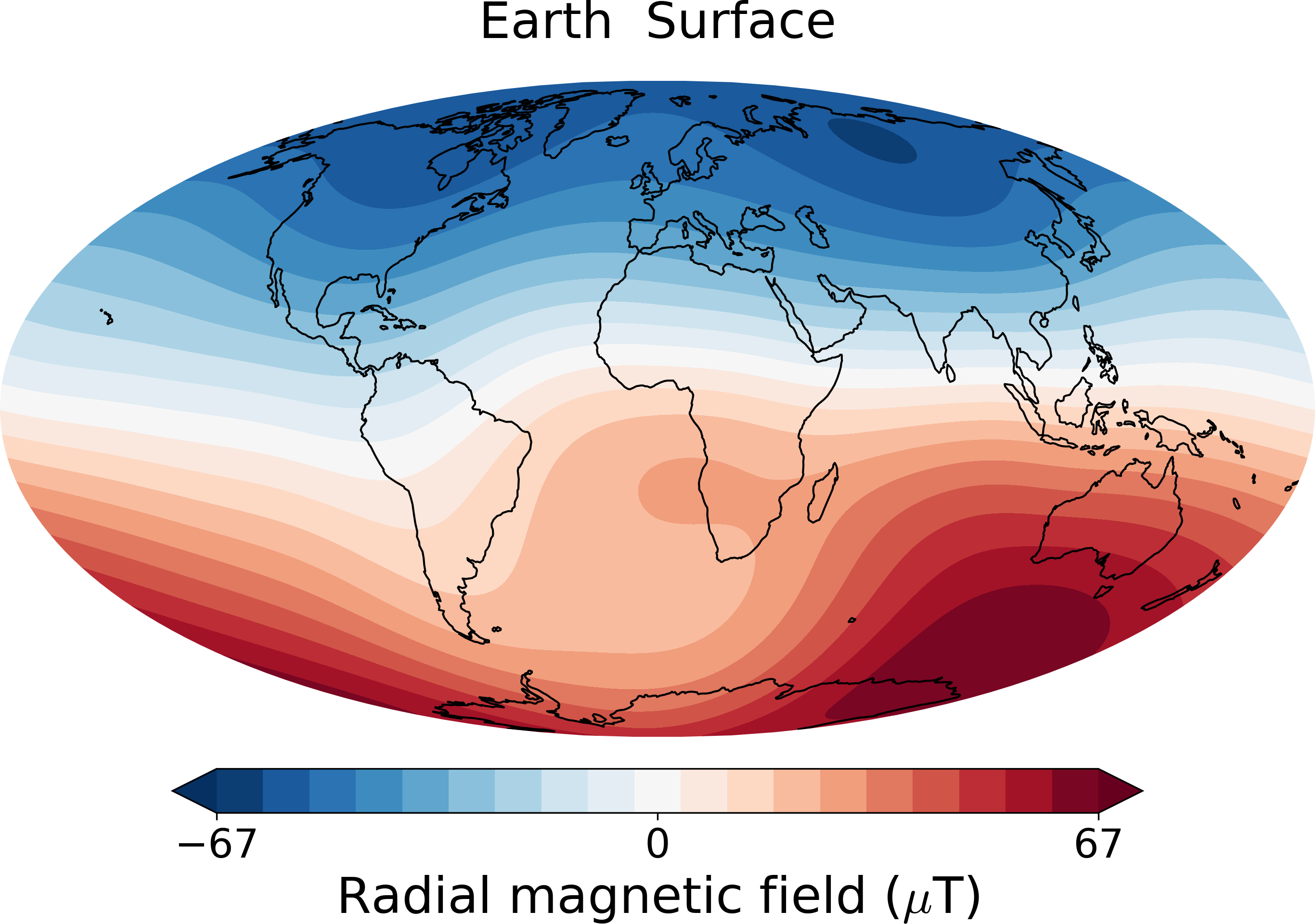
2.1.1. Planet.plot()

This function plots a 2D surface plot of the radial magnetic field at radius r given in terms of the surface radius. For example,

from planetmagfields import Planet
p = Planet(name='earth')
p.plot(r=1,proj='Mollweide')

produces the info mentioned above first and then the following plot of Earth’s magnetic field using a Mollweide projection

while

from planetmagfields import Planet
p = Planet(name='jupiter',model='jrm09')
p.plot(r=0.85,proj='Mollweide')

produces the following info about Jupiter and then plot that follows

Planet: Jupiter
l_max = 10
Dipole tilt (degrees) = 10.307870

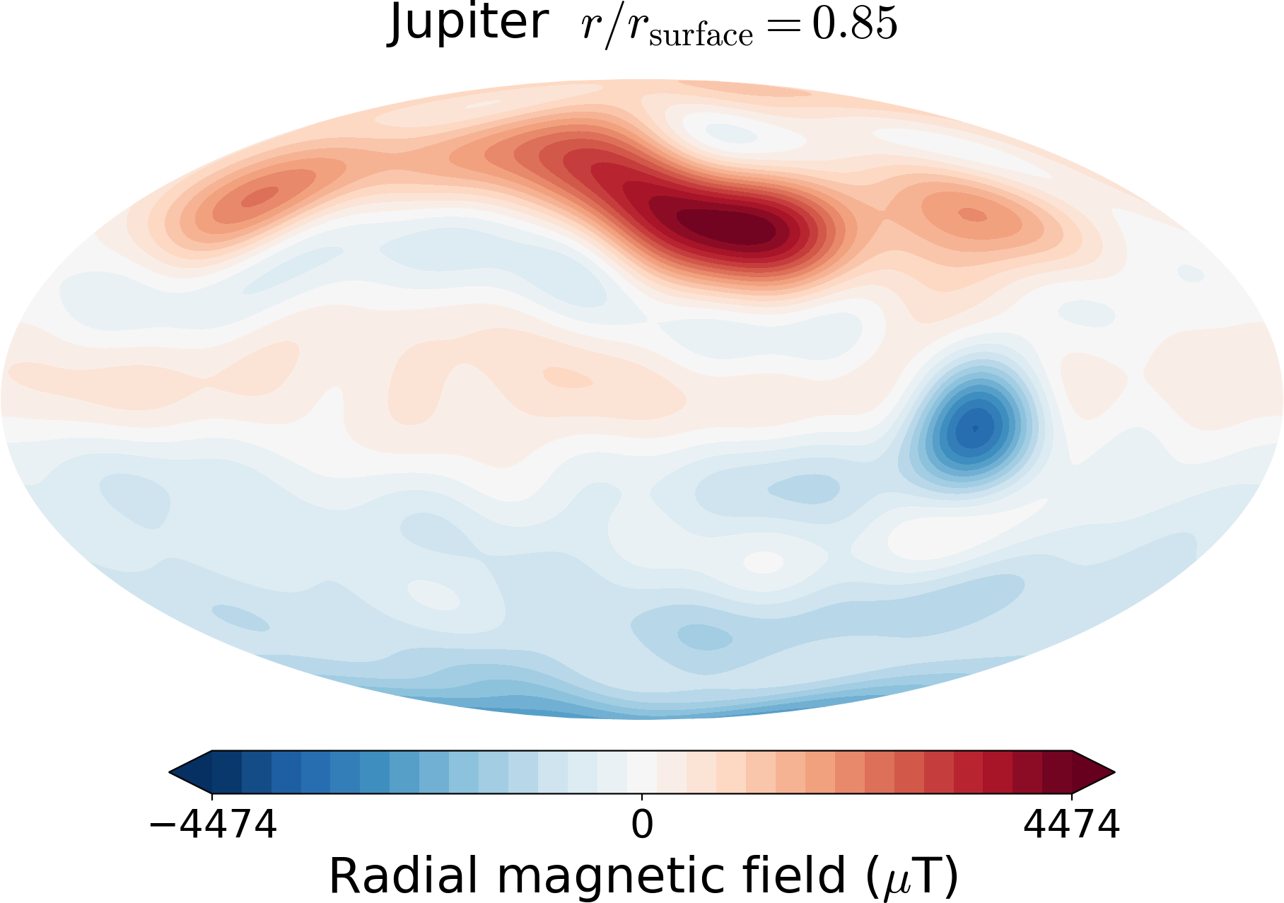
This can be compared with Fig. 1 g from Moore et al. 2018 .

2.1.2. Planet.spec()

This function computes the Lowes spectrum of a planet at a given radius. It adds an array p.emag_spec which contains the energy at different spherical harmonic degrees and two variables p.dipolarity and p.dip_tot which provide the fraction of energies in the axial dipole and the total dipole with respect to the total energy at all degrees. In addition, it provides equatorially symmetric and antisymmetric as well as axisymmetric contributions to the Lowes energy spectrum. Usage example:

from planetmagfields import Planet
p = Planet(name='jupiter',model='jrm33')
p.spec()

will provide variables

In [22]: p.dipolarity
Out[22]: 0.747204704567949

In [23]: p.dip_tot
Out[23]: 0.7719205020945153

In [24]: p.emag_spec
Out[24]:
array([0.00000000e+00, 3.47735401e+11, 2.36340427e+10, 2.12851283e+10,
      1.75661770e+10, 1.92219833e+10, 9.91200748e+09, 3.34535482e+09,
      3.95317968e+09, 2.59333418e+09, 1.23423771e+09])

In [25]: p.emag_symm/p.emag_tot # Symmetric part
Out[25]: 0.16062699807374292

In [26]: p.emag_antisymm/p.emag_tot # Anti-symmetric part
Out[26]: 0.8393730019262573

In [27]: p.emag_axi/p.emag_tot # Axisymmetric part
Out[27]: 0.7768733455808511

and will produce Jupiter’s surface spectrum:

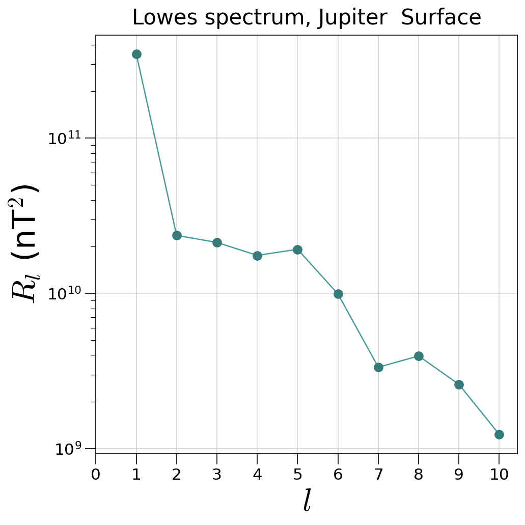
The plotting can be suppressed setting the logical p.spec(iplot=False). A different radius other than surface can be selected using the p.spec(r=0.8) parameter. API documentation : Planet.spec()

2.1.3. Planet.writeVtsFile()

This function writes a vts file that can be used to produce 3D visualizations of field lines with Paraview/VisIt. Usage:

p.writeVtsFile(potExtra=True, ratio_out=2, nrout=32)

where,

• potExtra : bool, whether to use potential extrapolation. This uses the SHTns library for spherical harmonic transforms.

• ratio_out: float, radius till which the field would be extrapolated in terms of the surface radius

• nrout: radial resolution for extrapolation

Example of a 3D image produced using Paraview for Neptune’s field, extrapolated till 5 times the surface radius is given below.

2.2. Field filtering using Planet.plot_filt

The planet class also provides a function for producing a filtered view of the radial magnetic field using the function plot_filt. This function can take in either an arbitrary array of spherical harmonic degrees and orders or cut-off values. This is illustrated below with examples, assuming the user is in the repository directory.

2.2.1. Saturn’s small-scale magnetic field

Here we plot Saturn’s magnetic field at a depth of 0.75 planetary radius for spherical harmonic degrees > 3.

from planetmagfields import Planet
p = Planet(name='saturn')
p.plot_filt(r=0.75,lCutMin=4,proj='Mollweide')

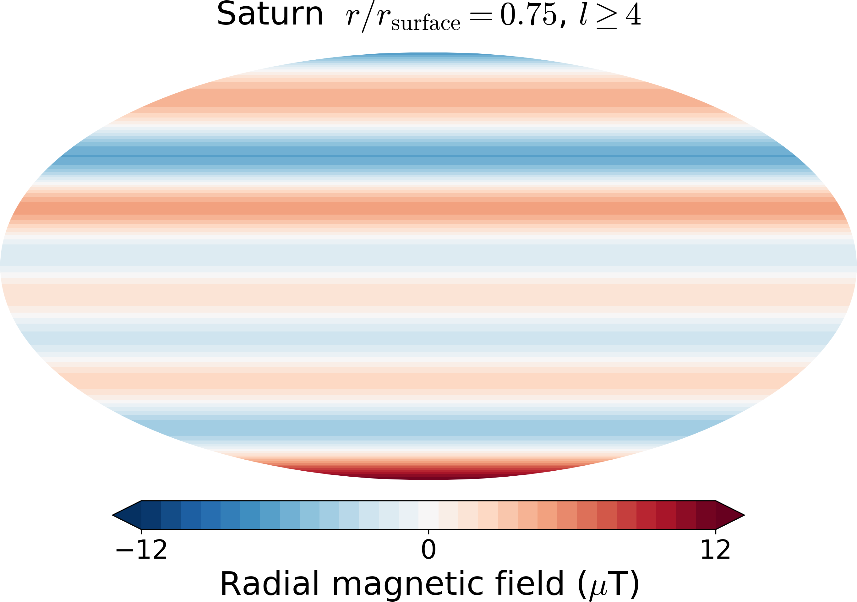
Compare this with Fig. 20 B from Cao et al. 2020 .

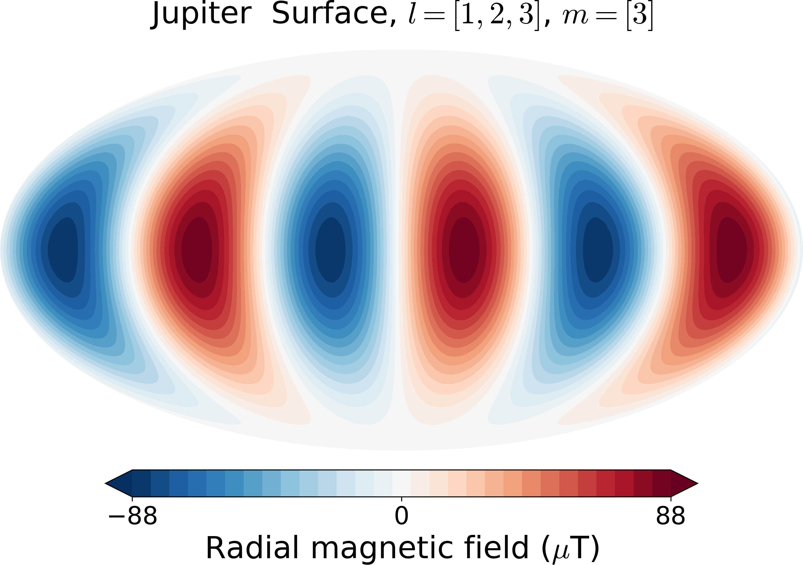
2.2.2. Jupiter’s surface field

Here we filter out Jupiter’s surface field restricted to degrees 1,2,3 and order 3.

from planetmagfields import Planet
p = Planet(name='jupiter',model='jrm09')
p.plot_filt(r=1,larr=[1,2,3],marr=[3],proj='Mollweide')

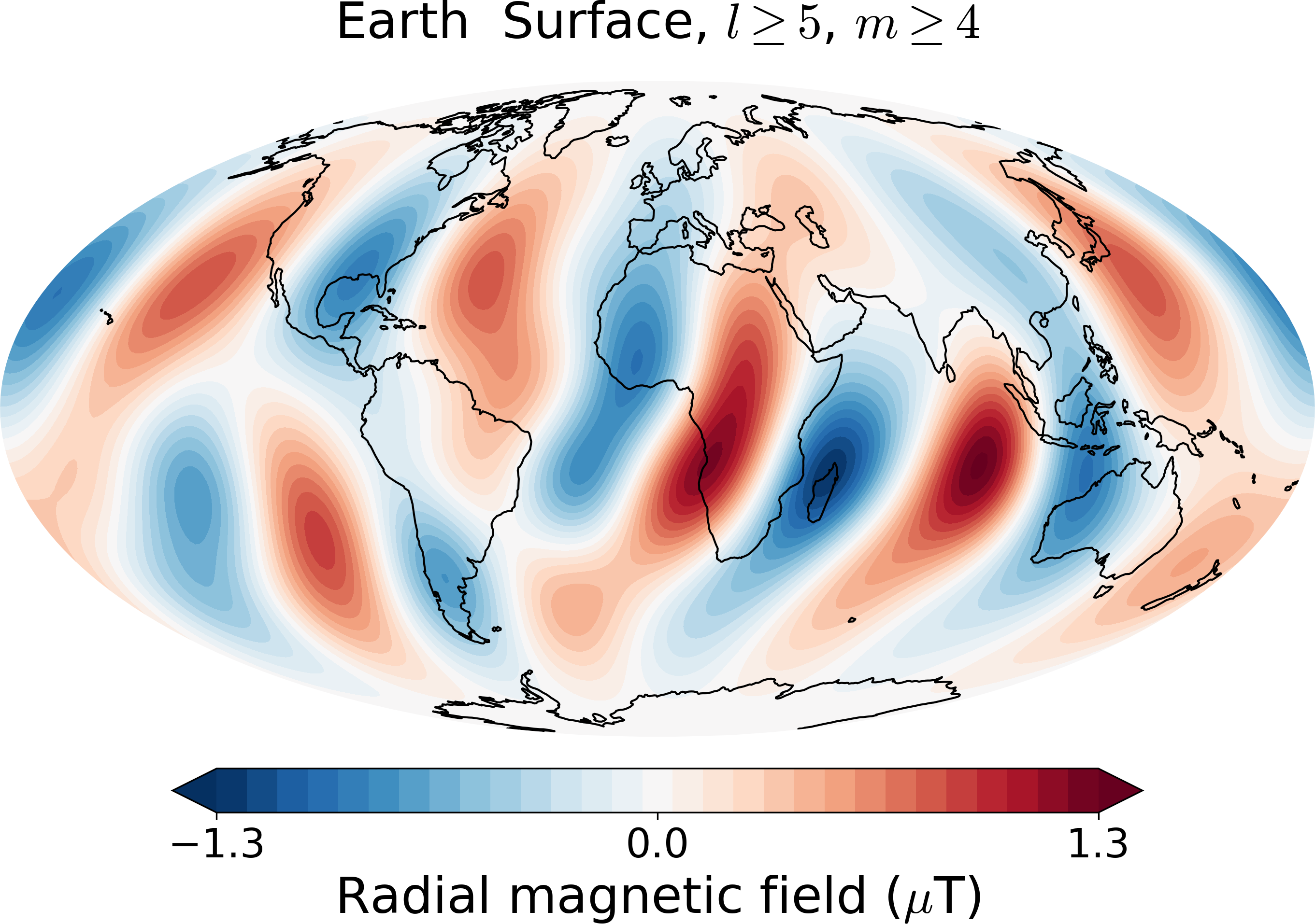
2.2.3. Earth’s smaller scale surface field

We filter the surface field to degrees > 4 and orders > 3.

from planetmagfields import Planet
p = Planet(name='earth')
p.plot_filt(r=1,lCutMin=5,mmin=4,proj='Mollweide')

2.3. Potential extrapolation

Warning

Potential extrapolation prior to v1.5.1 had a bug and the extrapolated fields would be overestimated. Please take care!

The Planet.extrapolate performs a potential extrapolation of a planet’s magnetic field. The functions are present in the potextra module. This uses the SHTns library for spherical harmonic transforms. Usage example:

import numpy as np
from planetmagfields import Planet
p = Planet('saturn')
ratio_out = 5 # Ratio (> 1) in terms of surface radius to which to extrapolate
nrout = 32 # Number of grid points in radius between 1 and ratio_out
rout = np.linspace(1,ratio_out,nrout)
p.extrapolate(rout) #Gives you three arrays p.br_ex, p.btheta_ex, p.bphi_ex

2.4. Get field along a trajectory

Warning

Potential extrapolation prior to v1.5.1 had a bug and the extrapolated fields would be overestimated. Please take care!

You can obtain field components along a trajectory (for example, obtained from NASA’s SPICE Toolkit) using the function Planet.orbit_path. This uses the SHTns library for spherical harmonic transforms but falls back to SciPy if SHTns is not available. Usage example below using some points from the Cassini Grand Finale:

from planetmagfields import Planet
p = Planet('saturn')

r = [17.82905598, 17.82110528, 17.81314499, 17.80517584, 17.79719656] # Can also be numpy array
theta = [1.1865416 , 1.18632847, 1.18611515, 1.18590167, 1.18568798]
phi = [4.70867942, 4.70884014, 4.70900102, 4.70916207, 4.7093233 ]

p.orbit_path(r,theta,phi)
print(p.br_orb)
print(p.btheta_orb)
print(p.bphi_orb)

This will provide the outputs:

Planet: Saturn
Model: cassini11+
l_max = 14
Dipole tilt (degrees) = 0.000000
[0.00278097 0.00278617 0.00279139 0.00279662 0.00280187]
[0.00347406 0.00347843 0.00348281 0.00348721 0.00349161]
[0. 0. 0. 0. 0.]

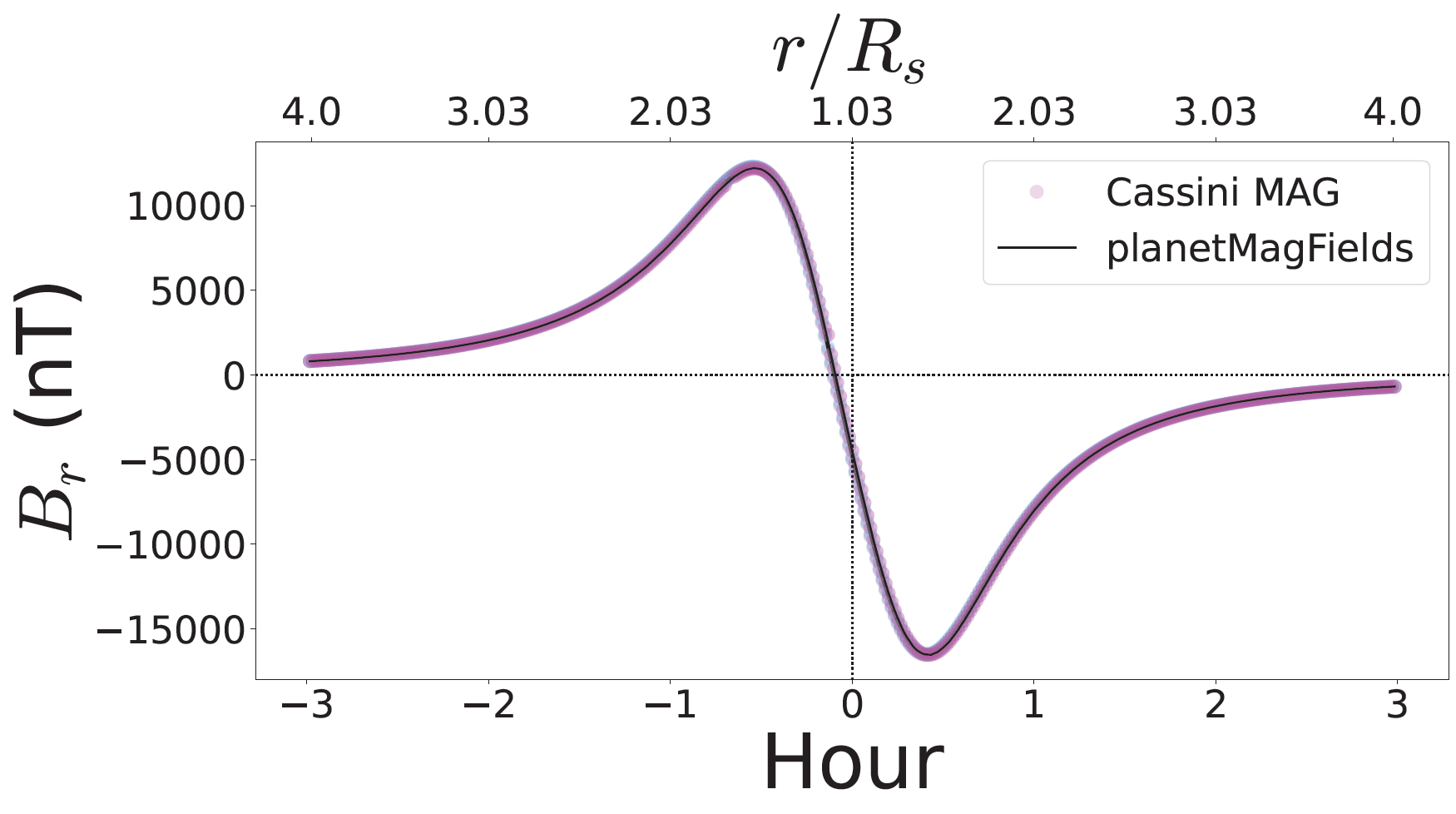
A plot for the Cassini Grand Finale trajectory compared against the MAG data is shown below:

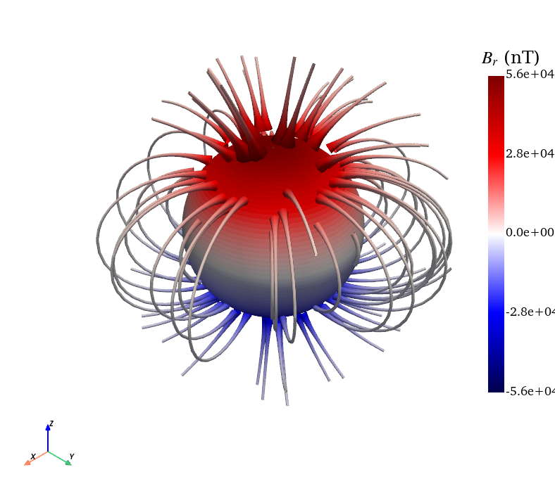
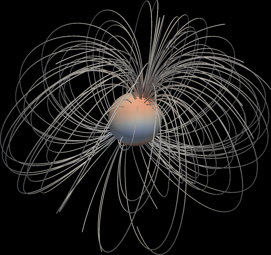
2.5. 3D Visualization with Planet.plot3D

The Planet.plot3D function allows for 3D visualization of a planet’s magnetic field. This can be particularly useful for understanding the spatial distribution and behavior of the magnetic field in three dimensions. This function makes use of VTK using the PyVista library. An example usage is shown below:

from planetmagfields import Planet
p = Planet('saturn')
p.plot3D(fieldlines=True)

which produces a 3D plot of the magnetic field lines for the planet Saturn.